Notes-on-Query-Execution:part1

SQL 是用户使用的，数据库会把 SQL 转换成某种内部表示，类似于扩展的关系代数。

关于词法、语法解析的部分，比较幸运的是，很多书都介绍了怎么处理 SQL:

• https://book.douban.com/subject/6109479/
• https://book.douban.com/subject/27082372/

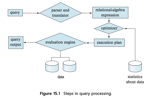
Query-evaluation Engine 处理给定的 Plan, 执行这个 Plan, 然后把结果返回给查询。

查询的代价

https://colin-scott.github.io/personal_website/research/interactive_latency.html

上面是每年的 Latency Numbers Every Programmer Should Know

2020 年：

1. Main memory reference: 100ns
2. SSD random read: 16000ns
3. 1,000,000 bytes sequentially from SSD: 49, 000ns
4. Disk seek: 2ms
5. 1,000,000 bytes sequentially from dosl: 825, 000 ns

书上作者举的是2018年的例子，HDD Seek + 传送数据可以以10ms为单位，SSD则快得多，经常处在亚0.1 ms 级。（结合我这边生产，感觉基本没有用 HDD 的了…不晓得存储会不会这么搞）

此外，有些东西会让这些统计变得更复杂：

1. 无论用 mmap 还是手写 buffer pool，读写的很大一部分势必在内存中
2. 如果系统有多个 disk, 那么并行访问多个 disk 可能能比在一个 disk 上 IO 快很多

下面介绍了 Postgres 的策略：

In addition, although we assume that data must be read from disk initially, it is possible that a block that is accessed is already present in the in-memory buffer. Again, for simplicity, we ignore this effect; as a result, the actual disk-access cost during the execution of a plan may be less than the estimated cost. To account (at least partially) for buffer residence, PostgreSQL uses the following “hack”: the cost of a random page read is assumed to be 1/10th of the actual random page read cost, to model the situation that 90% of reads are found to be resident in cache.

Selection

下面介绍一下 B+Tree 的一些参数：

1. $h_i$ B+Tree 的高度。
2. $t_s$ : block-access time (disk seek time plus rotational latency) ， 对于 SSD，2018 年大约是 90 microseconds；对于 HDD,2018 年大概是 4ms
3. $t_T$ 单个 block 数据传输的时间，对于 SSD，有 10 microseconds for a 4-kilobyte block. 对于 HDD，这个速度慢得多

（2021年还有人用 HDD 做 DB 吗？这也太慢了，氪金就是力量诶）

那么，开销大概是：

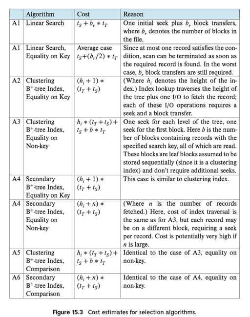
给出一个 A2 的参考 Cluster Index Equality on Key: $(h_i + 1) * (t_T + t_s)$ . 在 cluster index找到就可以，路径都需要读到。

A3 则是因为大概要找到 left-most page，然后执行 A1 类似的逻辑。以此类推。

有上述内容，我们大概可以知道 MySQL 里面查询、回表之类的代价估计了。

不过上述 cluster index 和 secondary index 就涉及到了索引选择的问题。如果满足要求的数据很多，那就直接走 cluster index 了，否则数据少的话走 secondary index 优化，岂不美哉。

Postgres 实现了 bitmap index scan, 走 index 挑出需要 scan 的 block, 再决定具体的行为。可以看：https://dba.stackexchange.com/questions/119386/understanding-bitmap-heap-scan-and-bitmap-index-scan

Conjunction/Disjunction/Negation

这…表面上懂的都懂，但这里涉及一个问题：假如有多于一个索引，索引选择怎么办

To reduce the cost, we choose a θi and one of algorithms A1 through A6 for which the combination results in the least cost for σθi (r). The cost of algorithm A7 is given by the cost of the chosen algorithm.

一种方式如上述 A7，根据 cost 选择一个代价最低的索引

另一种方式 A8 是走 composite index（中文似乎叫联合索引）。

A9 需要有对应的 UID 来做 tuple 标示，它会走多个索引，然后取相同的 uid。

Disjunction 需要所有的路径都可以走 index, 否则退化成 Linear Scan.

Sorting

(我感觉排序这种在面试里面出现过一万遍了，然后数据结构书一般都讲了外排序吧…)

$M$ 系统可以提供给 sort 的 block 数目

$b_b$ 被定义为 N-way Merge 阶段可以处理的 block 数目

$b_r$ 为这个 relation 的 block 数量

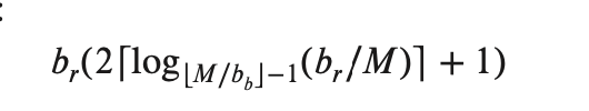
1. 第一次产生了 $b_r$ 的 block 输出，IO 大致为 $b_r / M$
2. 每一次能够处理 $M / b_b$ 次
3. 产生了上述结果

可以看看 TiDB 的外部排序：https://github.com/pingcap/tidb/issues/12431

Join

首先贴一下书上给的模型吧：

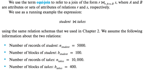
（想起了我们说唱大学，因为数据库没什么考的，所以要把书上给的 Schema 背下来，然后默写 SQL，真的傻逼）

Nested-loop join / Block Nested-loop join

真的有人在用吗…

简单说：Nest-loop Join 就是搞两个循环来 Join; Block Nest-loop Join 就是针对关系的 block 搞两个循环，内层走 nest-loop join.

不过值得注意的是，外层的 tuple 只会 Scan 一遍，内层的会 Scan 很多遍。理智告诉我们应该把内层的放小一点。

实际上，考虑到类似的场景，例如 broadcast join: https://jaceklaskowski.gitbooks.io/mastering-spark-sql/content/spark-sql-joins-broadcast.html 其实思路也差不多

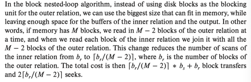
上述方法能够减少内层 IO ，因为我们一次性读取了多个外层 block, 减少了循环的次数。

Indexed Nested-loop Join

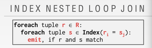
Although the number of block transfers has been reduced, the seek cost has actually increased, increasing the total cost since a seek is considerably more expensive than a block transfer. However, if we had a selection on the student relation that reduces the number of rows significantly, indexed nested-loop join could be significantly faster than block nested-loop join.

其实看上去有优势，但是并没有好多少。

Sort-Merge Join

这个去掉了 loop 的形式，采取 sort ，然后在有序的区间内作 equal 的操作。

Merge 的操作是 $M + N$, sort 的操作如之前所叙述。此外，在 worst case 中，如果两个关系中所有的 join key 都一样，那么 Merge 的操作会退化到 $M * N$

此外，有一种 Hybrid merge-join 的算法, 如果关系 A 走在 cluster index 或者已经有排序，关系 B 可以走 secondary index。那么可以 A 和 B merge, 再去 B 做类似 index bitmap scan 的操作。为什么需要这样呢？如果两边都是 secondary index 才能 Join 的话，可能会有莫名其妙的 IO 代价放大。

Hash Join

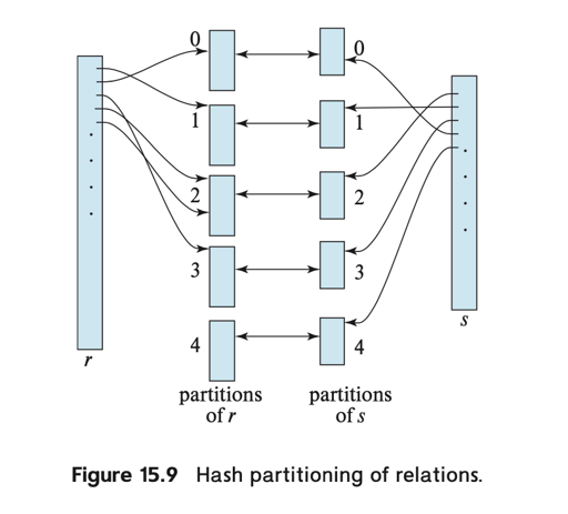
先看看书上的形式化定义：

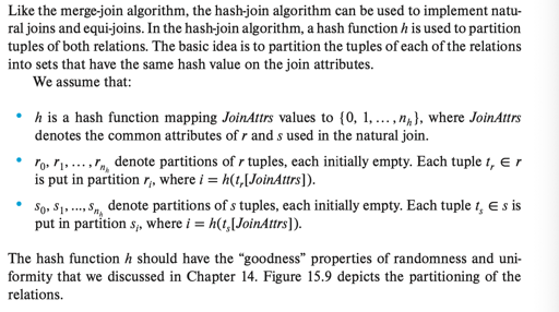
(实际上这里用的是 grace hash join)

这里分为 build phase 和 probe phase。如果 s 能装在内存中，那就直接在内存中哈希，然后扫 r。

否则给 s 和 r 构建 hash index, 然后每个相同的 hash 做 nested loop join 的操作。

这里问题是：

Skew/Overflow: 数据可能倾斜，这里可以避免产生过大的 block, 或者递归走 hash build

关于 hash join, 这里有一些性能分析：

对于 grace hash join, 每个 block 要：

1. 读取一遍，然后哈希写入一遍，这是一个 pass
2. 再读取一遍，做 nested loop join, 这是一个 pass

此外，哈希会造成 $n_h$ 的冗余 block 开销，所以，这里的开销是：

$3(b_r + b_s) + 4n_h$

在递归的情况下，我们要利用到因子 $M$ 得到：

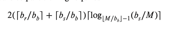
15-445 指出，一般来说 hash join 有着比较好的效率，不过已排序/要排序的数据，可以使用 sort join

如果内层关系很小，且外层可以走索引，那 Index Nested Loop Join 会不错，否则可以试试 Hash Join，这个应该需要根据统计信息来判定。

Hybrid Hash Join

hybrid hash join 做了内存足够的时候，执行上的优化，这里考虑的场景是「内存比较大，但是整个 Hash Join 也不是完全放得下」的场景。之前考虑过 s 全部构件在内存或者写到盘上的情况的情况，感觉 hybrid hash join 构建了一个半 on-disk hash，来优化这个操作。我们构造一个 $s_0$, 它包含:

• 先将一个关系切分成 t 在内存中，k - t 在盘上，然后哈希
• 另一个关系 load 起来 t 份和之前的关系直接处理，剩下的部分再走盘上哈希的流程。

以此来优化。

杂项：优化

使用 bloom filter 来优化 Join

其他运算

Duplicate Elimination

• 使用 hashing 或者 sorting 去重
• 有些 DB 有 HLL 之类的模糊手段

Set

大体是构建 hash map 甚至 on-disk hash, 然后 probe.

Aggregation

感觉是一个另类的统计，我实现的时候构建过一个统计的 hash, 统计完之后遍历取信息。这里有不同的方案：

1. 在构造过程中（类似流式的）取信息
2. 走 Hashing 来构造

正常情况下，能不 swap 到盘上还是不 swap 到盘上吧，但是算子之间肯定还是有区别的。

查询执行

15-445 应该介绍过 DB 的查询执行。比较传统的执行方式是 volcano 模型，这个模型和当时的硬件结构是有关的。同时，我们也知道 vectorize 和 codegen 等模型。我们可以在 MonetDB/X100 和 Efficiently Compiling Efficient Query Plans for Modern Hardware 这两篇论文找到对应的答案。

这里表达式执行可以分为：

1. 物化执行（materialized evaluation）：中间关系的结果需要被物化
2. 流水线执行（pipeline evaluation）：可以减少临时文件（物化输出）的数量，将结果能直接输出给下一个表达式。这种方式能够消除读写中间输出的代价。其中，也能够这样区分对应的输出方式
   1. 需求驱动：由 top 的算子来发送 next 或者 next_batch 这样的请求，驱动下层的算子来取对应的数据。可以看作是 pull 的模型
   2. 生产者驱动：底层的算子产生 tuple，然后输出给上层的算子。可以看作是 push 的模型

在查询中，可以流水化的边被称为 pipelined edge, 需要物化的（比如 Hash Join）被称为 blocking edge. 一般来说，不同的 pipeline edge 组成的子树可以并发执行，blocking 的可能需要物化。

这里还介绍了一下 streaming 上的查询执行，感觉可以看：https://www.skyzh.dev/posts/articles/2022-01-15-store-of-streaming-states/

此外，有些 cache 亲和的查询执行策略，这里是让划分的 block 能 fit 在 L1/L2/L3 cache 中，从而加速查询。

这里还介绍了查询编译和 columnar 执行，不过就提了两行。